How find duplicates in Google Sheets?

The COUNTIF or conditional formatting features coul be used how to find duplicates in Google Sheets. In today’s article we will look at this topic in more detail. But enough of the introduction, let’s solve duplicates from Sheets.

Use COUNTIF function to know if row is duplicate

To find duplicates in a Google Sheets spreadsheet, you can use the COUNTIF function to count the number of times a specific value appears in a range of cells. You can then use this information to identify duplicates.

Example of how you can use the COUNTIF function to find duplicates:

1. Select the range of cells that you want to search for duplicates in.
2. Click on an empty cell where you want to display the result of the COUNTIF function.
3. Type the following formula in the selected cell, replacing “A1:A10” with the range of cells you want to search and “A1” with the cell you want to count =COUNTIF(A1:A10, A1)
4. Press Enter to apply the formula.
5. The selected cell should now display the number of times the value in cell A1 appears in the range of cells you specified.
6. Repeat this process for each cell in the range you want to search for duplicates in. Any cells with a value greater than 1 indicate a duplicate.

The function for counting duplicates:

=COUNTIF(A1:A, A1)

The COUNTIF function is case-sensitive, so it will only count duplicates if the case of the text matches exactly. If you want to count duplicates regardless of case, you can use the COUNTIF function in combination with the UPPER or LOWER functions to convert the text to all uppercase or all lowercase before the duplicate count is performed.

How highlight duplicates in Google Sheets?

To highlight duplicates in a Google Sheets spreadsheet, you can use the built-in conditional formatting feature. Here’s how:

1. Select the range of cells that you want to highlight duplicates in.
2. Click the “Format” menu at the top of the screen, then click “Conditional formatting” in the drop-down menu.
3. In the “Format cells if” drop-down menu, select “Custom formula is”
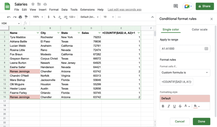
4. Type into code =COUNTIF(A1:A, A1)>1 into input.
5. Choose the formatting options you want to apply to the duplicates, such as the font color and fill color.
6. Click “Done” to apply the conditional formatting to the selected cells.

The selected cells should now be highlighted to indicate any duplicates. Note that the highlighting will only be applied to cells with duplicate values, not to cells with unique values.

The function to highlight duplicates:

=COUNTIF(A1:A, A1)>1

Real-life use

Below you can see how to use this functionality. Either in a column or in conditional formatting. Just be careful you need to set up the proper shift blocking with $ otherwise it won’t work.