Drop-down list in Google Sheets
Today I will show you the drop-down list feature in Google Sheets. How to create a “basic” drop-down list, how to create a drop-down list from other columns and I will show you some of the mine tips on how I work with them.
How create a basic drop-down list in Google Sheets?
Creating the drop-down list is easy and everyone could use it. There are two ways which you could use. The first one is to create a drop-down list from the static list. The second way is to create a dynamic drop-down from another column (and maybe in another tab).
Here’s a quick comparison of the two methods:
| Static method | From column |
|---|---|
| 🟢 much faster to implement | 🔴 you have to take care of the list |
| 🔴 editing means affecting the whole column | 🟢 works better in the longer term |
| 🟢 good for a newbie | 🟢 good for the experienced |
You can’t quite say use one or the other. Each path lends itself to something a little different, and besides how to create them during the article, hopefully, you’ll get a better understanding of what to use and when.
How create static drop-down list in Google Sheets?
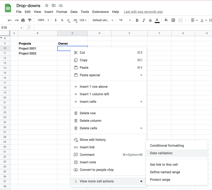
Create a “static” drop-down list when you know which options you need. First, you need to open the “data validation” option from the menu, which is located under the right button and is hidden under “view more cell actions”…
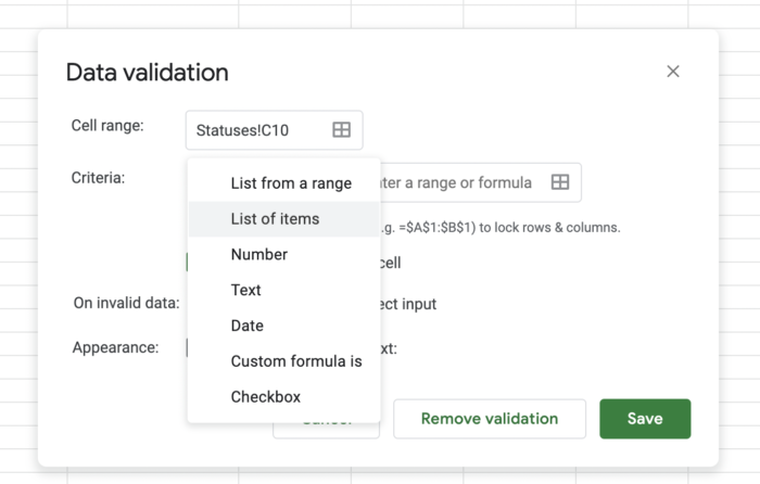
Then in “criteria”, you have to select the option “list of items” which sets just a static list. Don’t worry about the “list from ranges” option we will show below.
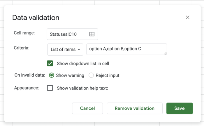
Now just add the sheet items to the pop-up and separate them with a comma (or semicolon) depending on what is written in the grey box. Try the following options:
option A, option B, option CFine, you can put a space between the comma and the next option. It should be automatically erased at the beginning and won’t get into the cells.
Now in the picture you can see what the basic drop-down list will look like:
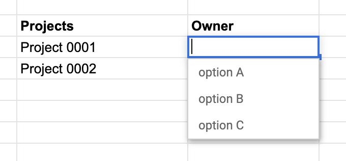
You can then “stretch” the sheet with a blue dot to other cells in a column or row to make more use of it.
How create a drop-down list from another column in Google Sheets?
Creating a sheet “from column” is practically the same as the above-described way. Only instead of “list of items” you choose “list of from range”. However, before doing so, I recommend creating a new sheet called settings where you will have your list set up.

If you choose “list from range” then you need to click on the table icon and then click in the box and expand the range where you have your values.
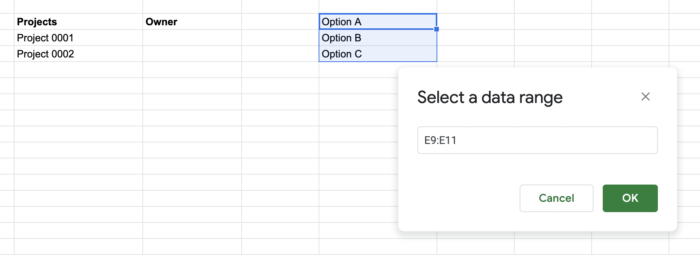
You can see that I have set E9:E11 but to make it work properly you need to set $E$9:$E$11 so that when you copy the range the data source does not change. Personally, I always delimit the cells and leave 3 spaces between the values so that I can insert new values. My settings sheet then looks like this:
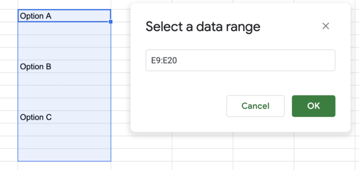
So it’s easier for me to edit the contents of the sheets. But that’s more of a hack of mine, and it’s not something that needs to be done.
How create a status drop-down list in Google Sheets?
If you want to create the status drop-down list you could create the basic drop-downs which about I wrote above. But you could add some emojis to your sheets. You could prepare a dynamic list that will look like this…
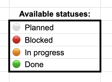
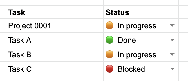
As you could see, I’ve used the circle’s emoji for a better understanding of the condition. Yes, you can use conditional formatting, but then your table might look very wild (full of colors) and you might not want that. In the picture below you can see what the statuses look like.
>> How do use emoticons to express task/project statuses? >>
Does vlookup work with drop-down lists in Google Sheets?
Yes if you use a drop-down list and after that, you want to get some number with vlookup so your patterns will work. You just want to make sure everything looks simple and you don’t get lost in the patterns later.

In the image above, you can see that vlookup works well in conjunction with the drop-down list. There is a sample that I have highlighted from Sheet which I use to connect salary from other columns…
=VLOOKUP(D3,$I$3:$J$5,2,false)… in D3 is the result of the drop-down list and with vlookup, I search this value in another list where I have my imaginal hourly salary in another column.
=VLOOKUP( what , where , column with data ,false)How add color to drop-down lists?
If you want use colors with drop-down lists in Google Sheets. You must use conditional formatting in the target column. If you set the background at the place from which you create the drop-down list, this background is not transferred to the target…

…but if you use conditional formatting as I wrote above your drop-down list could look much better or not? Below you can see what it can look like when I set the formatting. Yes, I put green on purpose to show that the red does not carry over anyway.
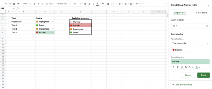
So if you want to color the results of the drop-down list you have to use conditional formatting.
How do I work with drop-down lists in Google Sheets?
Above I’ve outlined a few with the drop-down lists I’m working with. Realistically I rarely use them only when I’m sure I won’t need to add more items because then I would have to copy the drop-down list. Yes, I’m a bit lazy, but you have to be if you want to simplify your work.