IFERROR function in Google Sheets
Today we will look on function IFERROR which you should use in Google Sheets to fix #N/A as results of other functions. For me IFERROR function works well when I wrap a finished functions. Especially I use this function when I see that something breaks in result. Let’s see how you can use it.
To use the IFERROR function in Google Sheets, you would use the following syntax:
=IFERROR(formula, value_if_error)In code above “formula” is the formula that you want to evaluate, and “value_if_error” is the value that you want to display in the cell if an error occurs in the formula.
So I use this function only at the end when I have finished a complex formula. Especially when I notice that I have an incorrect output and it seems to me that it is not a problem of the pattern.
For example, suppose you have a formula that divides the value in cell A1 by the value in cell B1, but you want to display the text “Error” in the cell if either cell A1 or cell B1 contains an error or zero. You could use the following formula to achieve this:
=IFERROR(A1/B1, "Error")This formula would divide the values in cells A1 and B1, and display the result in the cell where the formula is entered. If either cell A1 or cell B1 contains an error or zero, the formula would display the text “Error” instead.
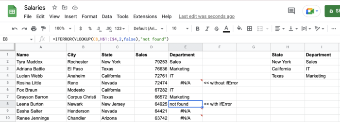
Using IFERROR on VLOOKUP results
The VLOOKUP function in Google Sheets allows you to search for a specific value in a range of cells and return a corresponding value from a different column in the same row. However, if the value you are searching for is not found in the range, the VLOOKUP function will return an error.
To avoid this error, you can use the IFERROR function to handle the error and display a more meaningful result in the cell. For example, suppose you have a table of data in cells A1 to C10, with the first column containing the values you want to search for, and the second and third columns containing the corresponding values you want to return.
=IFERROR(VLOOKUP(A1, A1:C10, 3, FALSE), "Not found")Most of the time when I use VLOOKUP I am pulling some values from a secondary table (for example, from the stats of previous year). Sometimes it happens that I don’t have a given value in the previous year, so I wrap VLOOKUP with IFERROR and I know that if I don’t find the given value I will get, for example, 0.
